Feature selection techniques
Published:
Notes on feature selection techniques
General notes
Supervised feature selection techniques consider the target variable when determining variable relevance
- Wrapper - Evaluate performance of model trained on subsets of input features and select features with greatest performance
- Filter - Feature selection based on relationship between feature and target variables
- Intrinsic - Automatically perform feature selection during training (e.g., Decision trees, LASSO)
Unsupervised feature selection techniques ignore the target variable and remove redundant variables (e.g., by using correlation)
Checking correlation to determine redundant redundant variables
Strong correlation between variables may indicate dependent relationships between variables or redundancy. It is best to remove these or reduce the number of them to avoid overfitting
Correlation metrics
Some useful measures of correlation are the Pearson’s correlation coefficient, Spearman’s rank correlation coefficient, and Kendall’s $\tau$ correlation coefficient (not discussed here yet)
Pearson’s correlation coefficient (linear) - Also called “correlation coefficient”, describes the linear correlation between two variables. The correlation coefficient between variables $X$ and $Y$, $\rho$, is
$$\rho_{X,Y}=cov(X,Y)/\sigma_X\sigma_Y$$
- \(cov\) is the covariance
- \(\sigma_X\) is the standard deviation of \(X\)
- \(\sigma_Y\) is the standard deviation of \(Y\)
The coefficient can have values of $-1\le\rho\le+1$. The larger the absolute value of $\rho$ (i.e., closer to $\pm1$), the more strongly correlated the two variables are. $\rho=0$ indicates no correlation, i.e., no linear dependence between the variables
Calculate the Pearson’s correlation coefficient in python with:
Spearman’s (rank) correlation coefficient (nonlinear) - A measure of monotonicity between linear or nonlinear variable. It is the Pearson correlation coefficient between the rank variables. Spearman’s correlation coefficient, $\rho_{R(X),R(Y)}$ or $r_s$, is calculated as
$$\rho_{R(X),R(Y)}=r_s=cov(R(X),R(Y))/\sigma_{R(X)}\sigma_{R(Y)}$$
- $\rho$ is the Pearson correlation coefficient applied to the rank variables
- $cov(R(X),R(Y))$ is the covariance of the rank variables
- $\sigma_{R(X)} and \sigma_{R(Y)}$ are the standard deviations of the rank variables
Calculate the Spearman’s rank correlation coefficient in python with:
Correlation strength is generally understood as
STRONG $$0.7\le|\rho|\le1.0$$ MODERATE $$0.3\le|\rho|<0.7$$ WEAK $$0.0\le|\rho|<0.3$$
Correlation plots
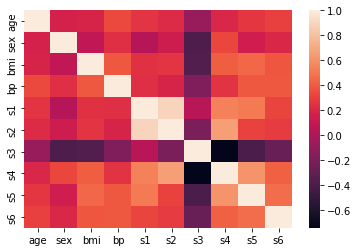
Correlation plots are a visual way to represent the correlation matrix, a table showing correlation coefficients between pairs of variables on the X and Y axes
Calculate the Pearson’s correlation coefficient matrix of a pandas dataframe object, df, with df.corr(method='pearson') or just df.corr()
Using the seaborn module, execute seaborn.heatmat(correlation_matrix)
A full example of calculating and plotting the correlation matrix of the sklearn diabetes dataset
# Import modules for handling dataframes and plotting
import pandas as pd, seaborn as sns

# Import the diabetes dataset module
from sklearn.dataseets import load_diabetes

# Load the diabetes dataset into a dataframe
data = load_diabetes(return_X_y=True, as_frame=True)[0]

# Calculate the correlation matrix of the dataframe
corr_mat = data.corr()

# Plot the correlation matrix as a heatmap
sns.heatmap(corr_mat)

Selection methods
Python modules can be used to automatically perform feature selection. Jason Brownlee for Machine Learning Mastery recommends the following two
- Select the top k variables: SelectKBest
- Select the top percentile variables: SelectPercentile
These must be paired with a scoring function (e.g., Pearson’s correlation coefficient, chi-squared, etc.)
References
Feature Engineering and Selection: A Practical Approach for Predictive Models
